kurtosis

function of dascore.transform.kurtosis

kurtosis(
    patch: Patch ,
    samples: bool = False,
    recursive: bool = True,
    **kwargs ,
)-> ‘PatchType’

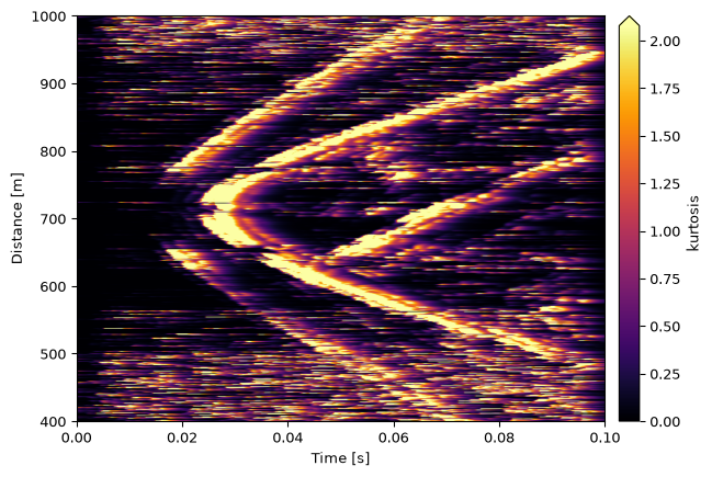
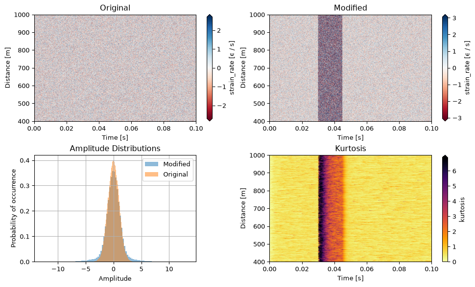
Compute kurtosis along a patch dimension. Background seismic noise is approximately Gaussian. A seismic arrival (especially a P-wave onset) produces a transient, impulsive signal with a sharply peaked amplitude distribution. Kurtosis — the normalized 4th statistical moment — becomes strongly positive during such impulsive arrivals.

Here, kurtosis is determined in a window whose length is given as a dimension keyword argument (e.g. time=0.5). We then determine kurtosis of the amplitude distribution in that window. Higher kurtosis thus indicates high amplitude outliers. This in turn can be interpreted as a signal arrival.

Parameters

Parameter	Description
patch	Input DASCore patch.
samples	If True, the values in kwargs and step represent samples along a dimension. Must be integers. Otherwise, values are assumed to have same units as the specified dimension, or have units attached.

recursive	If True, use recursive pseudo-kurtosis: Instead of computing kurtosis in a sliding window (computationally expensive for continuous data), Langet et al. (2014) propose a recursive formulation. This acts like an exponentially weighted moving estimator, so the algorithm updates continuously without storing long windows of data. If False, the common kurtosis calculation is used
**kwargs	Used to specify the dimension and window length, e.g. `time=0.5` computes kurtosis in 0.5 second windows along the time dimension. Units are also supported, e.g. `distance=10 * dascore.units.get_unit('m')`.

Returns

PatchType A new patch with kurtosis traces.

Examples

import dascore as dc

p = dc.examples.get_example_patch('example_event_2')

k = p.kurtosis(time=0.002)
ax = k.viz.waterfall(cmap = 'inferno')
import dascore as dc
import numpy as np
import matplotlib.pyplot as plt

p = dc.examples.get_example_patch('example_event_2')

# replace event data with normal-distributed random values
rng = np.random.default_rng()
data = rng.normal(loc=0, scale=1, size=p.data.shape)
data0 = data.copy() # original
data[:,300:450] = data[:, 300:450]*3 #modified

orig = p.update(data=data0)
modi = p.update(data=data)

# calculate kurtosis on modified data
k = modi.kurtosis(time=0.002)

fix, axs = plt.subplots(2,2, figsize=(10,6), layout='constrained')
ax = orig.viz.waterfall(cmap = 'RdBu', ax=axs[0,0])
_ = ax.set_title('Original')

ax = modi.viz.waterfall(cmap = 'RdBu', ax=axs[0,1])
_ = ax.set_title('Modified')

ax = k.viz.waterfall(cmap = 'inferno_r', scale=[0, .4], ax=axs[1,1])
_ = ax.set_title('Kurtosis')

# plot histograms of both datasets. Note the modified has broader tail!
_ = axs[1,0].hist(data.ravel(),  100, alpha=0.5, label='Modified', density=True)
_ = axs[1,0].hist(data0.ravel(), 100, alpha=0.5, label='Original', density=True)
_ = axs[1,0].legend(loc='upper right')
_ = axs[1,0].grid('on')
_ = axs[1,0].set_title('Amplitude Distributions')
_ = axs[1,0].set_xlabel('Amplitude')
_ = axs[1,0].set_ylabel('Probability of occurrence')

References

Langet, Nadège, Alessia Maggi, Alberto Michelini, and Florent Brenguier. 2014. “Continuous Kurtosis-Based Migration for Seismic Event Detection and Location, with Application to Piton de la Fournaise Volcano, La Réunion.” Bulletin of the Seismological Society of America, 229–46. https://doi.org/10.1785/0120130107.